Some notes on practical PEPA modelling

In order to understand what follows, you should be comfortable with the following topics:

• Properties of the exponential distribution and Poisson processes [2].
• Homogeneous Continuous Time Markov Chains [2].
• PEPA process algebra [1].

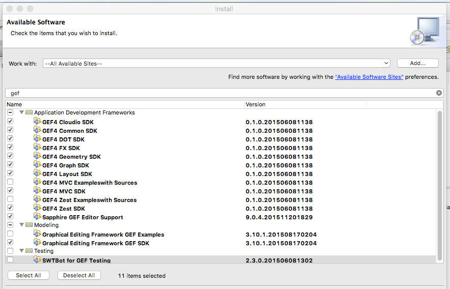
You should also install the PEPA Plug-in Project in Eclipse.
Note: when you add the PEPA software source to Eclipse, use the following repository URL, which always points to the latest release: http://www.dcs.ed.ac.uk/pepa/group/updatesite/ . You should also install GEF and Zest components, as shown below

Notice that, if you are using our department's laboratories, you don't need to perform the previous actions, as you could simply run C:\eclipsePEPA\eclipse if you are using Windows, or /opt/shared/x86_64/eclipse-pepa/eclipse if you are using Linux.

Once you have started Eclipse, click on Window menu → Open Perspective → Other → PEPA.

Now you're ready to create a new project: click on File menu → New → Project → General → Project, then click on Next. Choose whichever project name you want and then click on Finish.

In order to create a new file with your PEPA model, from the navigator panel (on the left side of the window), right-click on the project you have created, and then click on New → Other → General → File, then click on Next. Choose the file name you want, but be sure to append the .pepa extension at the end of the name, then click on Finish.

Models can be expressed writing the appropriate PEPA encoding in the created .pepa file using the editor window (the middle one). Please refer to [1] for the syntax and the semantics of PEPA operators. Mind, however, that there are some differences between the PEPA syntax on paper and the one that you should use here. More specifically:

• Comment lines begin with //.
• Each statement must end with a semicolon ; .
• You can define numerical constants, that can later be used as rates, as name = value.
• The prefix ( (type,rate).P ) and the choice ( P + Q ) operators behave as usual.
• The undefined rate (top) is represented either by T or infty.
• Component definition (def) is represented by the = sign.
• The synchronisation/cooperation operator between P and Q over a set of action types a_1,..,a_n is represented by P <a_1,…,a_n> Q.
• Parallel composition, i.e., < > can also be represented by ||.
• Parallel composition of identical processes, i.e., P || … || P can also be written as P[n], where n is the number of identical components.
• The last statement of the file must be a system equation, i.e. a cooperation or a parallel composition, without the ending semicolon.

Consider a really basic system architecture in which there is a client and a server. The client performs requests to the server and then wait for an answer. The server, in turn, wait for requests, and then answer at his own pace.

In order to model the system using PEPA, we need to make some (completely arbitrary) assumptions, i.e.,

• The client cannot perform requests while it is waiting for an answer.
• The client can perform only a single request at time.
• The server can satisfy only a single request at time, and only when the client has asked for that.

queue1.pepa

l = 3.0; // arrival rate
m = 5.0; // service rate
n=1; // number of servers

// arrival process
A = (a,l).A;

// server
S = (s,m).S;

// queue, c = 10
Q00 = (a,T).Q01;
Q01 = (a,T).Q02 + (s,T).Q00;
Q02 = (a,T).Q03 + (s,T).Q01;
Q03 = (a,T).Q04 + (s,T).Q02;
Q04 = (a,T).Q05 + (s,T).Q03;
Q05 = (a,T).Q06 + (s,T).Q04;
Q06 = (a,T).Q07 + (s,T).Q05;
Q07 = (a,T).Q08 + (s,T).Q06;
Q08 = (a,T).Q09 + (s,T).Q07;
Q09 = (a,T).Q10 + (s,T).Q08;
Q10 =             (s,T).Q09; // blocking behaviour

A <a> Q00 <s> S[n]

queue2.pepa

// simpler encoding of two m/m/1/c
l = 2.0; // arrival rate
m1 = 5.0; // service rate of the first queueing centre
m2 = 3.0; // service rate of the second one

// first queue, c = 5
Q0 = (a,l).Q1;
Q1 = (a,l).Q2 + (s,m1).Q0;
Q2 = (a,l).Q3 + (s,m1).Q1;
Q3 = (a,l).Q4 + (s,m1).Q2;
Q4 = (a,l).Q5 + (s,m1).Q3;
Q5 =            (s,m1).Q4;

// another queue, c=3
S0 = (s,T).S1;
S1 = (s,T).S2 + (d,m2).S0;
S2 = (s,T).S3 + (d,m2).S1;
S3 =            (d,m2).S2;

Q0 <s> S0

gc.pepa

// garbage collection

// gc activation rate
ga_r = 1.0;
// gc deactivation rate
gd_r = 5.0;

// gc collection rate
gc_r = 30.0;

// arrival rate
l = 5.0;
// service rate (mem free)
m = 20.0;

// gc
GC_OFF = (s,T).GC_OFF + (ga,ga_r).GC_ON;
GC_ON = (gc,gc_r).GC_ON + (gd,gd_r).GC_OFF;

// memory, 4 blocks
MEM0 = (s,m*1.00).MEM0 + (a,T).MEM1;
MEM1 = (s,m*0.75).MEM1 + (a,T).MEM2 + (gc,T).MEM0;
MEM2 = (s,m*0.50).MEM2 + (a,T).MEM3 + (gc,T).MEM1;
MEM3 = (s,m*0.25).MEM3 + (a,T).MEM4 + (gc,T).MEM2;
//MEM4 =                   (a,T).MEM4 + (gc,T).MEM3; // non-blocking arrival
MEM4 =                                (gc,T).MEM3; // blocking arrival

// queue
Q0 = (a,l).Q1;
Q1 = (a,l).Q2 + (s,T).Q0;
Q2 = (a,l).Q3 + (s,T).Q1;
Q3 = (a,l).Q4 + (s,T).Q2;
Q4 = (a,l).Q5 + (s,T).Q3;
Q5 = (a,l).Q6 + (s,T).Q4;
Q6 = (a,l).Q7 + (s,T).Q5;
Q7 = (a,l).Q8 + (s,T).Q6;
Q8 = (a,l).Q9 + (s,T).Q7;
Q9 = (a,l).Q10+ (s,T).Q8;
Q10 =           (s,T).Q9;

GC_OFF <gc,s> MEM0 <a,s> Q0

philisophers.pepa

// the random philosophers problem
// (first) fork catching rate
r_fc = 1.0;
// (first) fork releasing (dining) rate
r_fr = 5.0;
// second fork catching and releasing (almost immediate)
r_fci = 1000.0;
r_rfi = 1000.0;

// forks, released and caught
F1R = (fc1,T).F1C;
F1C = (fr1,T).F1R;

F2R = (fc2,T).F2C;
F2C = (fr2,T).F2R;

F3R = (fc3,T).F3C;
F3C = (fr3,T).F3R;

F4R = (fc4,T).F4C;
F4C = (fr4,T).F4R;

F5R = (fc5,T).F5C;
F5C = (fr5,T).F5R;

// i-th philosopher, meditating, with left fork (i), right fork (i+1%5) and dining
P1M = (fc1,r_fc).P1L +
	  (fc2,r_fc).P1R;
P1L = (fc2,r_fci).P1D;
P1R = (fc1,r_fci).P1D;
P1D = (fr1,r_fr).P1DL +
      (fr2,r_fr).P1DR;
P1DL= (fr2,r_rfi).P1M;
P1DR= (fr1,r_rfi).P1M;

P2M = (fc2,r_fc).P2L +
	  (fc3,r_fc).P2R;
P2L = (fc3,r_fci).P2D;
P2R = (fc2,r_fci).P2D;
P2D = (fr2,r_fr).P2DL +
      (fr3,r_fr).P2DR;
P2DL= (fr3,r_rfi).P2M;
P2DR= (fr2,r_rfi).P2M;

P3M = (fc3,r_fc).P3L +
	  (fc4,r_fc).P3R;
P3L = (fc4,r_fci).P3D;
P3R = (fc3,r_fci).P3D;
P3D = (fr3,r_fr).P3DL +
      (fr4,r_fr).P3DR;
P3DL= (fr4,r_rfi).P3M;
P3DR= (fr3,r_rfi).P3M;

P4M = (fc4,r_fc).P4L +
	  (fc5,r_fc).P4R;
P4L = (fc5,r_fci).P4D;
P4R = (fc4,r_fci).P4D;
P4D = (fr4,r_fr).P4DL +
      (fr5,r_fr).P4DR;
P4DL= (fr5,r_rfi).P4M;
P4DR= (fr4,r_rfi).P4M;

P5M = (fc5,r_fc).P5L +
	  (fc1,r_fc).P5R;
P5L = (fc1,r_fci).P5D;
P5R = (fc5,r_fci).P5D;
P5D = (fr5,r_fr).P5DL +
      (fr1,r_fr).P5DR;
P5DL= (fr1,r_rfi).P5M;
P5DR= (fr5,r_rfi).P5M;

(F1R || F2R || F3R || F4R || F5R) <fc1,fc2,fc3,fc4,fc5,fr1,fr2,fr3,fr4,fr5> (P1M || P2M || P3M || P4M || P5M)

philisophers-nod.pepa

// the random philosophers problem, with no deadlocks
// (first) fork catching rate
r_fc = 4.0;
// (first) fork releasing (dining) rate
r_fr = 4.0;
// releasing rate of the first fork if the second is not taken
// (avoid deadlocks)
r_ad = 1.0;
// second fork catching and releasing (almost immediate)
r_fci = 1000.0;
r_rfi = 1000.0;

// forks, released and caught
F1R = (fc1,T).F1C;
F1C = (fr1,T).F1R;

F2R = (fc2,T).F2C;
F2C = (fr2,T).F2R;

F3R = (fc3,T).F3C;
F3C = (fr3,T).F3R;

F4R = (fc4,T).F4C;
F4C = (fr4,T).F4R;

F5R = (fc5,T).F5C;
F5C = (fr5,T).F5R;

// i-th philosopher, meditating, with left fork (i), right fork (i+1%5) and dining
P1M = (fc1,r_fc).P1L +
	  (fc2,r_fc).P1R;
P1L = (fc2,r_fci).P1D +
	  (fr1,r_ad).P1M;
P1R = (fc1,r_fci).P1D +
	  (fr2,r_ad).P1M;
P1D = (fr1,r_fr).P1DL +
      (fr2,r_fr).P1DR;
P1DL= (fr2,r_rfi).P1M;
P1DR= (fr1,r_rfi).P1M;

P2M = (fc2,r_fc).P2L +
	  (fc3,r_fc).P2R;
P2L = (fc3,r_fci).P2D +
	  (fr2,r_ad).P2M;
P2R = (fc2,r_fci).P2D +
	  (fr3,r_ad).P2M;
P2D = (fr2,r_fr).P2DL +
      (fr3,r_fr).P2DR;
P2DL= (fr3,r_rfi).P2M;
P2DR= (fr2,r_rfi).P2M;

P3M = (fc3,r_fc).P3L +
	  (fc4,r_fc).P3R;
P3L = (fc4,r_fci).P3D +
	  (fr3,r_ad).P3M;
P3R = (fc3,r_fci).P3D +
	  (fr4,r_ad).P3M;
P3D = (fr3,r_fr).P3DL +
      (fr4,r_fr).P3DR;
P3DL= (fr4,r_rfi).P3M;
P3DR= (fr3,r_rfi).P3M;

P4M = (fc4,r_fc).P4L +
	  (fc5,r_fc).P4R;
P4L = (fc5,r_fci).P4D +
	  (fr4,r_ad).P4M;
P4R = (fc4,r_fci).P4D +
	  (fr5,r_ad).P4M;
P4D = (fr4,r_fr).P4DL +
      (fr5,r_fr).P4DR;
P4DL= (fr5,r_rfi).P4M;
P4DR= (fr4,r_rfi).P4M;

P5M = (fc5,r_fc).P5L +
	  (fc1,r_fc).P5R;
P5L = (fc1,r_fci).P5D +
	  (fr5,r_ad).P5M;
P5R = (fc5,r_fci).P5D +
	  (fr1,r_ad).P5M;
P5D = (fr5,r_fr).P5DL +
      (fr1,r_fr).P5DR;
P5DL= (fr1,r_rfi).P5M;
P5DR= (fr5,r_rfi).P5M;

(F1R || F2R || F3R || F4R || F5R) <fc1,fc2,fc3,fc4,fc5,fr1,fr2,fr3,fr4,fr5> (P1M || P2M || P3M || P4M || P5M)

gc.pepa

// garbage collection

// gc activation rate
ga_r = 1.0;
// gc deactivation rate
gd_r = 5.0;

// gc collection rate
gc_r = 30.0;

// arrival rate
l = 5.0;
// service rate (mem free)
m = 20.0;

// gc
GC_OFF = (s,T).GC_OFF + (ga,ga_r).GC_ON;
GC_ON = (gc,gc_r).GC_ON + (gd,gd_r).GC_OFF;

// memory, 4 blocks
MEM0 = (s,m*1.00).MEM0 + (a,T).MEM1;
MEM1 = (s,m*0.75).MEM1 + (a,T).MEM2 + (gc,T).MEM0;
MEM2 = (s,m*0.50).MEM2 + (a,T).MEM3 + (gc,T).MEM1;
MEM3 = (s,m*0.25).MEM3 + (a,T).MEM4 + (gc,T).MEM2;
//MEM4 =                   (a,T).MEM4 + (gc,T).MEM3; // non-blocking arrival
MEM4 =                                (gc,T).MEM3; // blocking arrival

// queue
Q0 = (a,l).Q1;
Q1 = (a,l).Q2 + (s,T).Q0;
Q2 = (a,l).Q3 + (s,T).Q1;
Q3 = (a,l).Q4 + (s,T).Q2;
Q4 = (a,l).Q5 + (s,T).Q3;
Q5 = (a,l).Q6 + (s,T).Q4;
Q6 = (a,l).Q7 + (s,T).Q5;
Q7 = (a,l).Q8 + (s,T).Q6;
Q8 = (a,l).Q9 + (s,T).Q7;
Q9 = (a,l).Q10+ (s,T).Q8;
Q10 =           (s,T).Q9;

GC_OFF <gc,s> MEM0 <a,s> Q0

Consider a queueing system like the one of the Queueing Centre example. You have to modify it in order to model a system in which the processor can have multiple power states, e.g., high, low and off, which, of course, influence the performances of the cpu and its energy consumption. You have to make several assumptions on the power management behaviour of the system. After you have completed the model and computed the usual rewards (throughput, utilisation, etc.), try to answer to the following questions

• How we can automatically compute the power consumption of the system, given a set of parameters?
• How we can compute the energy efficiency of the system?
• How is it possible to compute the average latency W (expected response time E[R]), knowing the Little's law L=XW, where L is the average number of customers in the system and X is its throughput?

mmq.pepa

// markov modulated queue
// a sistem with 3 power state: high, low, stop
// service rates for high and low
m_h = 10;
m_l = 3;

// transition rate between high and low
r_hl = 1;
// transition rate between high and stop
r_hs = 0.05;
// transition rate between low and high
r_lh = 0.8;
// transition rate between low and stop
r_ls = 0.1;
// transition rate between stop and high
r_sh = 0.8;

// arrival rate
l = 2.0;

// modulating process
MHigh = (s,m_h).MHigh + 
		(t_hl,r_hl).MLow +
		(t_hs,r_hs).MStop;

MLow  = (s,m_l).MLow  +
		(t_lh,r_lh).MHigh +
		(t_ls,r_ls).MStop;

MStop = (t_sh,r_sh).MHigh;

S = (s,T).S;

// arrival process
A = (a,l).A;

// queue, c = 10
Q00 = (a,T).Q01;
Q01 = (a,T).Q02 + (s,T).Q00;
Q02 = (a,T).Q03 + (s,T).Q01;
Q03 = (a,T).Q04 + (s,T).Q02;
Q04 = (a,T).Q05 + (s,T).Q03;
Q05 = (a,T).Q06 + (s,T).Q04;
Q06 = (a,T).Q07 + (s,T).Q05;
Q07 = (a,T).Q08 + (s,T).Q06;
Q08 = (a,T).Q09 + (s,T).Q07;
Q09 = (a,T).Q10 + (s,T).Q08;
Q10 =             (s,T).Q09; // blocking behaviour

A <a> Q00 <s> S <s> MHigh

See Andrea Marin's example.

1. J. Hillston. A Compositional Approach to Performance Modelling. Cambridge University Press, 1996.
2. William J. Stewart. Probability, Markov Chains, Queues, and Simulation. Princeton University Press, 2009.